How to do multivariate time series forecasting in BigQuery ML
Companies across industries rely heavily on time series forecasting to project product demand, forecast sales, project online subscription/cancellation, and for many other use cases. This makes time series forecasting one of the most popular models in BigQuery ML.
What is multivariate time series forecasting? For example, if you want to forecast ice cream sales, it is helpful to forecast using the external covariant “weather” along with the target metric “past sales.” Multivariate time series forecasting in BigQuery lets you create more accurate forecasting models without having to move data out of BigQuery.
When it comes to time series forecasting, covariates or features besides the target time series are often used to provide better forecasting. Up until now, BigQuery ML has only supported univariate time series modeling using the ARIMA_PLUS model (documentation). It is one of the most popular BigQuery ML models.
While ARIMA_PLUS is widely used, forecasting using only the target variable is sometimes not sufficient. Some patterns inside the time series strongly depend on other features. Google see strong customer demand for multivariate time series forecasting support that allows you to forecast using covariate and features.
Google recently announced the public preview of multivariate time series forecasting with external regressors. Google are introducing a new model type ARIMA_PLUS_XREG, where the XREG refers to external regressors or side features. You can use the SELECT statement to choose side features with the target time series. This new model leverages the BigQuery ML linear regression model to include the side features and the BigQuery ML ARIMA_PLUS model to model the linear regression residuals.
The ARIMA_PLUS_XREG model supports the following capabilities:
- Automatic feature engineering for numerical, categorical, and array features.
- All the model capabilities of the ARIMA_PLUS model, such as detecting seasonal trends, holidays, etc.
Headlight, an AI-powered ad agency, is using a multivariate forecasting model to determine conversion volumes for down-funnel metrics like subscriptions, cancellations, etc. based on cohort age.
The following sections show some examples of the new ARIMA_PLUS_XREG model in BigQuery ML. In this example, we explore the bigquery-public-data.epa_historical_air_quality dataset, which has daily air quality and weather information. We use the model to forecast the PM2.51 , based on its historical data and some covariates, such as temperature and wind speed.
An example: forecast Seattle’s air quality with weather information
Step 1. Create the dataset
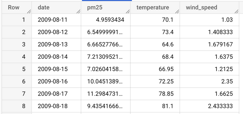
The PM2.5, temperature, and wind speed data are in separate tables. To simplify the queries, create a new table by joining those tables into a new table “bqml_test.seattle_air_quality_daily,” with the following columns:
- date: the date of the observation
- PM2.5: the average PM2.5 value for each day
- wind_speed: the average wind speed for each day
- temperature: the highest temperature for each day
The new table has daily data from 2009-08-11 to 2022-01-31.
CREATE TABLE `bqml_test.seattle_air_quality_daily`
AS
WITH
pm25_daily AS (
SELECT
avg(arithmetic_mean) AS pm25, date_local AS date
FROM
`bigquery-public-data.epa_historical_air_quality.pm25_nonfrm_daily_summary`
WHERE
city_name = 'Seattle'
AND parameter_name = 'Acceptable PM2.5 AQI & Speciation Mass'
GROUP BY date_local
),
wind_speed_daily AS (
SELECT
avg(arithmetic_mean) AS wind_speed, date_local AS date
FROM
`bigquery-public-data.epa_historical_air_quality.wind_daily_summary`
WHERE
city_name = 'Seattle' AND parameter_name = 'Wind Speed - Resultant'
GROUP BY date_local
),
temperature_daily AS (
SELECT
avg(first_max_value) AS temperature, date_local AS date
FROM
`bigquery-public-data.epa_historical_air_quality.temperature_daily_summary`
WHERE
city_name = 'Seattle' AND parameter_name = 'Outdoor Temperature'
GROUP BY date_local
)
SELECT
pm25_daily.date AS date, pm25, wind_speed, temperature
FROM pm25_daily
JOIN wind_speed_daily USING (date)
JOIN temperature_daily USING (date)
Here is a preview of the data:
Step 2. Create Model
The “CREATE MODEL” query of the new multivariate model, ARIMA_PLUS_XREG, is very similar to the current ARIMA_PLUS model. The major differences are the MODEL_TYPE and inclusion of feature columns in the SELECT statement.
CREATE OR REPLACE
MODEL
`bqml_test.seattle_pm25_xreg_model`
OPTIONS (
MODEL_TYPE = 'ARIMA_PLUS_XREG',
time_series_timestamp_col = 'date',
time_series_data_col = 'pm25')
AS
SELECT
date,
pm25,
temperature,
wind_speed
FROM
`bqml_test.seattle_air_quality_daily`
WHERE
date
BETWEEN DATE('2012-01-01')
AND DATE('2020-12-31')
Step 3. Forecast the future data
With the created model, you can use the ML.FORECAST function to forecast the future data. Compared to the ARIMA_PLUS model, you have to specify the future covariates as an input.
SELECT
*
FROM
ML.FORECAST(
MODEL
`bqml_test.seattle_pm25_xreg_model`,
STRUCT(30 AS horizon),
(
SELECT
date,
temperature,
wind_speed
FROM
`bqml_test.seattle_air_quality_daily`
WHERE
date > DATE('2020-12-31')
))
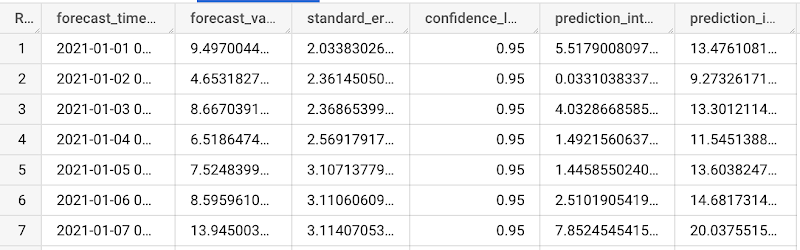
After running the above query, you can see the forecasting results:
Step 4. Evaluate the model
You can use the ML.EVALUATE function to evaluate the forecasting errors. You can set perform_aggregation to “TRUE” to get the aggregated error metric or “FALSE” to see the per timestamp errors.
SELECT
*
FROM
ML.EVALUATE(
MODEL `bqml_test.seattle_pm25_xreg_model`,
(
SELECT
date,
pm25,
temperature,
wind_speed
FROM
`bqml_test.seattle_air_quality_daily`
WHERE
date > DATE('2020-12-31')
),
STRUCT(
TRUE AS perform_aggregation,
30 AS horizon))
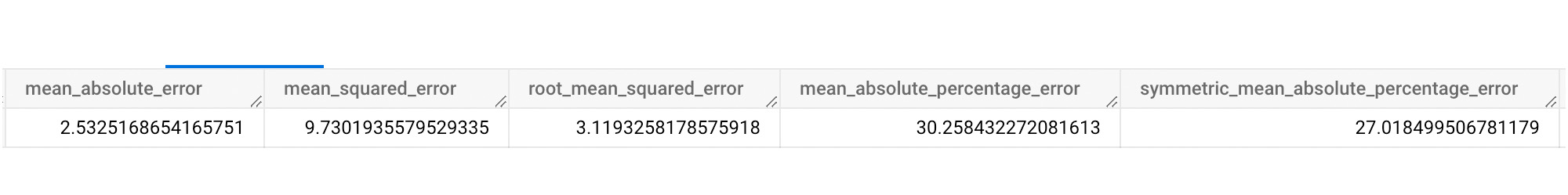
The evaluation result of ARIMA_PLUS_XREG is as follows:
As a comparison, we also show the univariate forecasting ARIMA_PLUS result in the following table:
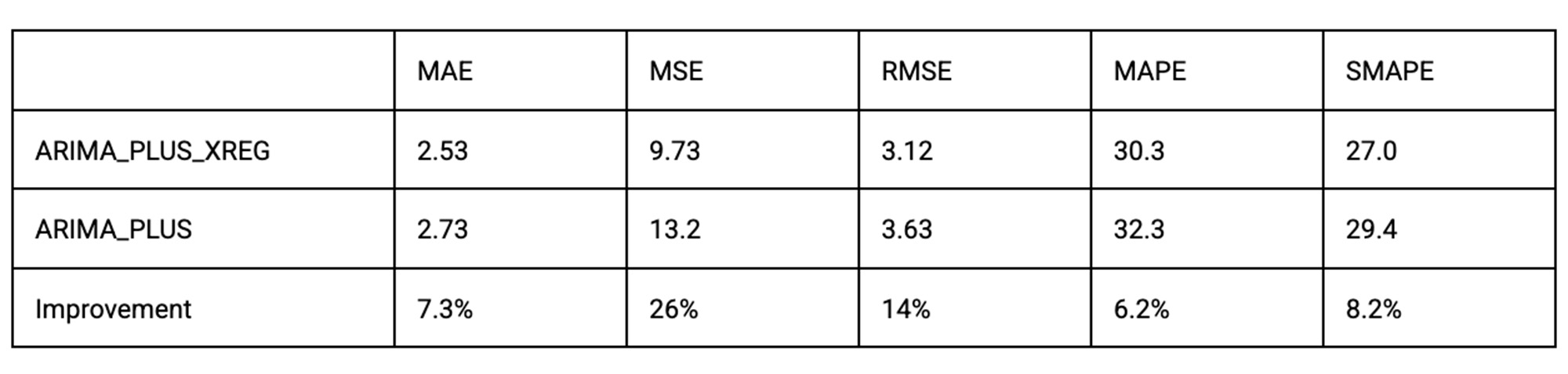
Compared to ARIMA_PLUS, ARIMA_PLUS_XREG performs better on all measured metrics on this specific dataset and date range.
Conclusion
In the previous example, Google demonstrated how to create a multivariate time series forecasting model, forecast future values using the model, and evaluate the forecasted results. The ML.ARIMA_EVALUATE and ML.ARIMA_COEFFICIENTS table value functions are also helpful for investigating your model. Based on the feedback from users, the model does the following to improve user productivity.
- It shortens the time spent preprocessing data and lets users keep their data in BigQuery when doing machine learning.
- It reduces overhead for the users who know SQL to do machine learning work in BigQuery.